The Cubix user's guide#
The graphical interface#
Cubix allows to make \(\gamma\)-ray spectroscopy analysis from histograms stored in ROOT files.
To start Cubix, simply use the command cubix
cubix
   ______        __     _       | Documentation: https://cubix.in2p3.fr/
  / ____/__  __ / /_   (_)_  __ |
 / /    / / / // __ \ / /| |/_/ | Source: https://gitlab.in2p3.fr/ip2i_gamma/cubix/cubix
/ /___ / /_/ // /_/ // /_>  <   |
\____/ \____//_____//_//_/|_|   | Version 1.0

[==        ] Loading tkn db...
 The loading of the TkN database is launched in a separate thread at cubix launch. It should take ~15 seconds (if not compiled in Debug) but it's not affecting the cubix usage.
This will open the Cubix main window as bellow:
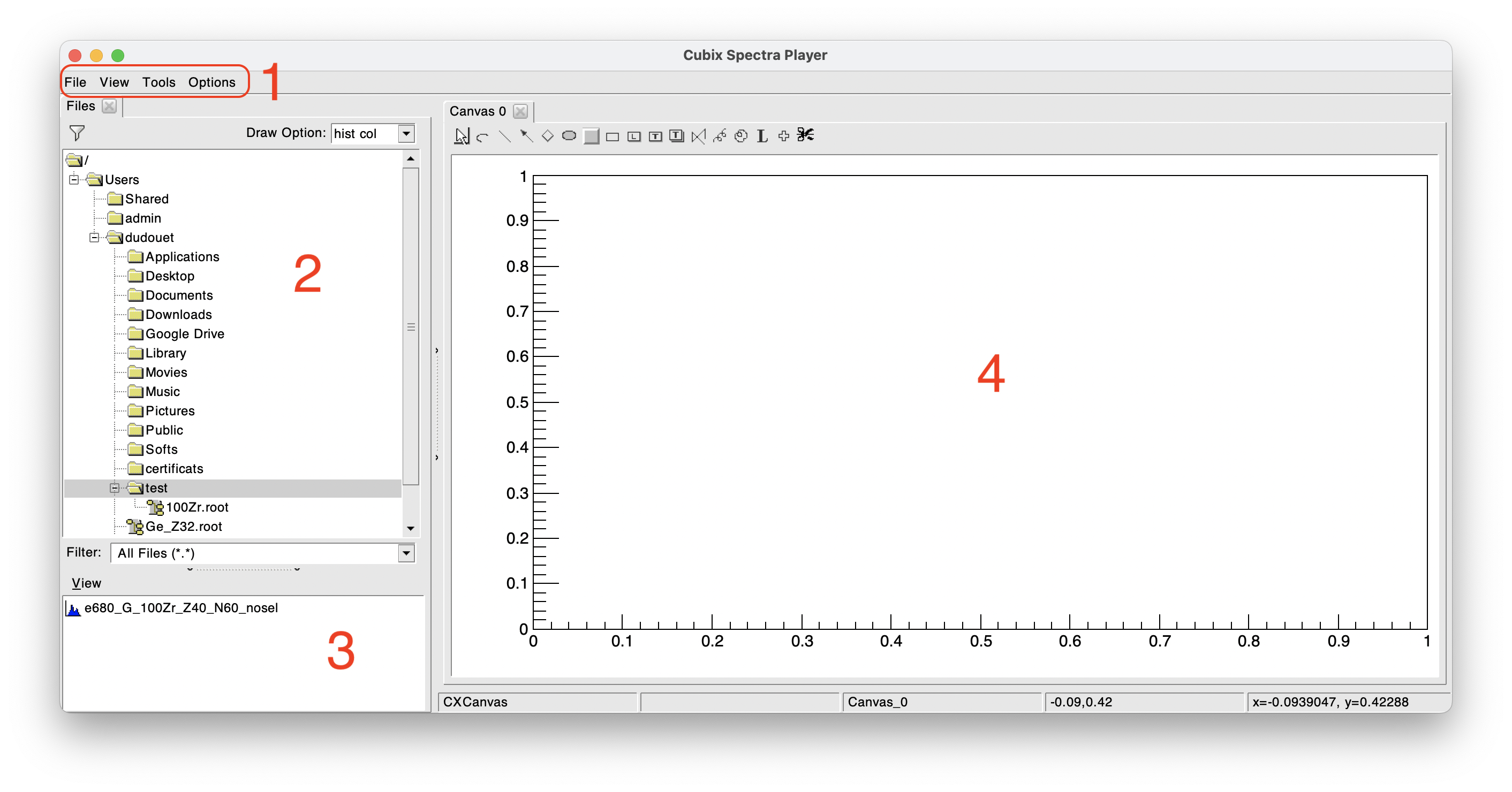
The Cubix main window is composed of different parts:
The Menu Bar#
The menu bar is composed of the following parts:
- The File menu:
- New Canvas: add a new active canvas to the display part
- New muti-pad Canvas: add a new active multi pad canvas (open a dialog box asking for number of X and Y pads)
- New Browser: open a standard ROOT TBrowser
- Save Canvas as: save the active canvas in the desired format (png, pdf...)
- Save hist to ASCII: save the active histogram in an ASCII file
- Exit: exit cubix
- The View menu:
- Browse Files: Open the file browser (part 2 on above picture)
- Saved list: Open the histogram saved list (see bellow)
- Workspace manager: Open the workspace manager (see bellow)
- Show editor: Open the ROOT editor
- Tools: These elements are described in detail in the following
- Options:
- Show stats: to display or not the spectra statistics
- Show Title: to display or not the spectra titles
The file browser#
By default, the left panel is dedicated to the file browser. It allows to navigate in your directories to find your favourite root file and open it (double click).
The file content will be displayed in the ROOT file browser (bottom left part). In this example (figure above), the opened ROOT file contains one 1D histogram.
To display a spectrum, double click on it. Using a right click on 1D/2D histograms, some shortcuts can be available for fits, background analysis or \(\gamma-\gamma\) analysis.
The saved list utility#
During an analysis, it can be useful to save spectra, for being reused or for being saved on disk. Any spectrum can be added to this list (right click: Add to stored spectra). This is in particular useful when doing \(\gamma-\gamma\) analysis to save the different projections.
In the following example, we can see that 3 spectra have been added to the saved list. It is then possible to write these spectra on disk using the "Save" button

The Workspace manager#
The workspace manager allows to create different workspaces for the analysis. A workspace is in general corresponding to an experiment configuration.
A workspace can contain:
- Energy calibration properties:
- graphical plot E (keV) vs E (channels) on which the calibration has been performed
- energy calibration function
- energy calibration error band (95% confidance level) calculated in the fit process
- residual plot resulting from the calibration process
- Efficiency properties:
- efficiency graph on which the fit has been performed
- efficiency function
- efficiency error band (95% confidance level) calculated in the fit process
- Energy resolution properties:
- FWHM graph on which the fit has been performed
- FWHM function
- FWHM error band (95% confidance level) calculated in the fit process
- Angular correlations:
- Geometrical correction factors (Q2/Q4) to be applied to angular correlation measurements
The way to create these files is explained in the following sections.
In the following example, we can see the Workspace manager window, where two workspaces are loaded in Cubix: E680 and SourceRun. The efficiency of the workspace SourceRun is plotted (graph + function + error band).

To create a new workspace, click on New workspace and enter the workspace name. It will create the workspace with all entries defined as None. To fill the workspace, refer to the sections Energy calibration, Efficiency fit or Angular correlations
The content of a workspace can be plotted by clicking on the workspace name and double clicking on its different elements.
To load a workspace, select it by clicking on the workspace name and then click on Load. The workspace will then be printed as Current Workspace in the workspace manager. For exemple, in the figure above, the current workspace is E680, even if the workspace displayed in the bottom left part is SourceRun.
Once a workspace is loaded, its properties will be used in the different Cubix tools:
- The calibration function can be used to calibrate a raw spectrum,
- The efficiency function is used to correct the peak area obtained from the peak fit utility,
- The FWHM function can be used to:
- automatically adapt the width of the gates to the detector resolution,
- constrain the FWHM in the peak fit utility to the detector resolution.
The principle of the Cubix workspace manager is to be able to keep all these information even after closing Cubix. All these properties are thus stored on disk in the Workspace directory. By default, the workspace directory is located in ${HOME}/Cubix_Workspaces.
If a file named .cubixrc is found in the ${HOME}, it is read to configure the workspace manager. This file should be like the following:
**********************************
***  Cubix configuration file  ***
**********************************

# This file can be copied in the ${HOME} to be automatically read by cubix

# Cubix Workspace define the folder in which the experiment workpaces are stored

CXWorkspace ${HOME}/Softs/Cubix/Workspaces

# Default_WS design the workspace to be loaded by default when launching cubix

Default_WS E680
- The entry corresponding to CXWorkspace refer to the location where the workspaces will be stored.
- The Default_WS defines, if filled, the workspace that is loaded by default when launching cubix.
The workspace directory can also be used to store some specific results from cubix like fit results.
Plotting histograms#
Draw options#
To plot an histogram, one just have to double click on it. It will be displayed using the Draw Option written on the top of panel 2.
The draw options are the standard ones from ROOT, with few more possibilities
- norm: Normalize the histogram in area,
- add: add the histogram to the current one,
- add(2) will add the histogram with factor 2,
- div: divide the histogram with the current one,
- div(2) will divide the histogram with factor 2,
- mult: multiply the histogram with the current one,
- mult(2) multiply the histogram with factor 2,
The Draw options can be added: ex: "hist norm same" will draw the selected histogram, normalised, on the same pad than the current histogram.
Histogram manipulations#
Histograms can be cut/copy/paste from one canvas to another. Right click on the histogram and select cut/copy, and then on another canvas, right click: paste.
An histogram can be removed from the current pad without being deleted, for this use right click: Undraw
An histogram already plotted in the canvas can be normalized or scaled using right click: Normalize/Scale
If the cursor is on an histogram, pressing SHIFT + wheel up/down scale up/down the histogram.
A raw histogram can be calibrated (if the calibration function has been defined in the current Workspace), using right click: Apply calibration
Zoom utilities#
Some tools have been added to the standard ROOT possibilities.
-
With the Shift key staying pressed, a click+slide with the mouse will draw a box on the canvas. When releasing the mouse click, the x range of the box will be applied to the histogram
-
With the Shift key pressed, a click on the canvas will make the range between zero and the clicked energy value.
-
With the Shift key pressed, a double click will unzoom the x axis.
-
On multi-pads Canvases, adding Ctrl+Shift apply the same zoom on all the pads.
-
When a zoom is applied on the X-axis (for 1D) or X and Y (for 2D), the keybord arrows allow to move on the histogram with the same zoom.
-
The wheel up/down allow on 1D histogram to zoom in/out on the Y axis (the cursor needs to be anywhere but not on an axis).
-
A X-axis range can be saved using z and applyed on an other one using Z.
Keyboard shortcuts#
A large number of keyboard shortcuts are available.
There is one known issue with keyboard shortcuts.
It a text zone has been clicked (like Draw Options, ENSDF nuclei...), instead of applying the keyboard shortcut, it will write the text in the text entry. This issue cannot be fixed. The only known solution for this is to switch to another window (like the terminal), and switch again on the cubix window to recover the ability of using keyboard shortcuts.
Find bellow the list of available shortcuts:
| Key | Result |
|---|---|
| CTRL+i | Print the shortcuts info in the terminal |
| Histogram manipulation | |
| CTRL+c | Copy histogram under cursor |
| CTRL+x | Cut histogram under cursor (copy and undraw) |
| CTRL+v | Paste the copied histogram in the current canvas (add to current ones) |
| CTRL+d | Undraw histogram under cursor |
| SHIFT+s | Add the spectrum under the cursor to the saved list |
| CTRL+n | Normalize histogram under cursor in area |
| CTRL+m | Normalize histogram under cursor to the maximum |
| SHIFT+wheel | Scale histogram under cursor |
| Canvas manipulation | |
| n | Open a new canvas |
| CTRL+g | set/unset grid on X and Y axes |
| SHIFT+c | set/unset CrossHair (wheel click to measure distances) |
| CTRL+u | Update canvas |
| z | Save the current X-axis range |
| Z | Apply the saved X-axis range |
| F12 | Unzoom |
| F9 | set/unset log scale on X axis |
| F10 | set/unset log scale on Y axis |
| F11 | set/unset log scale on Z axis |
| Arrows | Move on axis under cursor |
| Peak utilities | |
| s | Peak search (see Peak fitter section) |
| f | Start a new fit definition (see Peak fitter section) |
| CTRL+f | Perform the fit for the selected peaks (or double click) |
| CTRL+a | Start the calibration utility |
| c | Clear current fits and peak search values |
| r | Remove the arrow (from peak search or ENSDF) under the cursor |
| Gamma-Gamma mode | |
| g | Add a gate |
| g+g | Add a gate (open a dialog to set energy and width) |
| b | Add a background |
| b+b | Add a background (open a dialog to set energy and width) |
| c | Clear all gates and background |
| d | Remove the gate under the cursor |
| p | Project |
1D spectra utilities#
ENSDF reader#
The ENSDF reader allows to read, from the TkN library, all ENSDF/XUNDL databases and to plot on top of the displayed histogram arrows corresponding to the known transitions.
Write the name of the nucleus you want to plot and press enter to validate. This will gives something as:

By default, the ENSDF dataset "ADOPTED LEVELS, GAMMAS" is used. This contains all the known gamma rays, combining all the nucleus production methods (\(\beta\)-decay, coulex, fission...). This is possible to select the desired dataset using the ENSDF data-set list. In the following figure, the dataset has been changed to Uranium fission, limitating drastically the number of \(\gamma\)-rays.

In this last plot, the option "Full title" has been used to print more information on the \(\gamma\)-rays. Some parameters can be used to filter the type of decays to be shown.
Peak fitter#
The Peak fitter utility is composed of four sub parts:
- Peak search:
The peak search is a one-dimensional peak search tool based on the ROOT TSpectrum class.
Sigma is the sigma of searched peaks while threshold remove all peaks with amplitude less than threshold*highest_peak

If you change the parameters, remember to clear the present peaks (Clear button) before starting a new search.
- Minimizer:
The two last utilities are based on ROOT fits. The minimizer allows to define which minimize will to be used for the fits. The Fit options can contain any options from ROOT standard fit options. The default value "I" is to use the integral of the function in the bin instead of the default bin center value. For more details on the options, see the ROOT documentation.
- Background Fit:
The background fit is a tool to be used when the statistics is too low to perform a good fit. The idea is to determine a range before and after the peak (four arrows) that will be used to fit the backgroud. The peak area is then determined using the histogram area minus the area of the fitted background.
If the efficiency function has been defined in the current Workspace, the area will also be printed corrected from the detector's efficiency. The position of the maximum in the fit range will be used for the energy determination.
To define the background ranges, click on Set and define the four limits of the background (2 arrows for the range before the peak and two after). Two types of background can be used, a 1rst order polynomial and/or and exponential function. Then click on Fit:
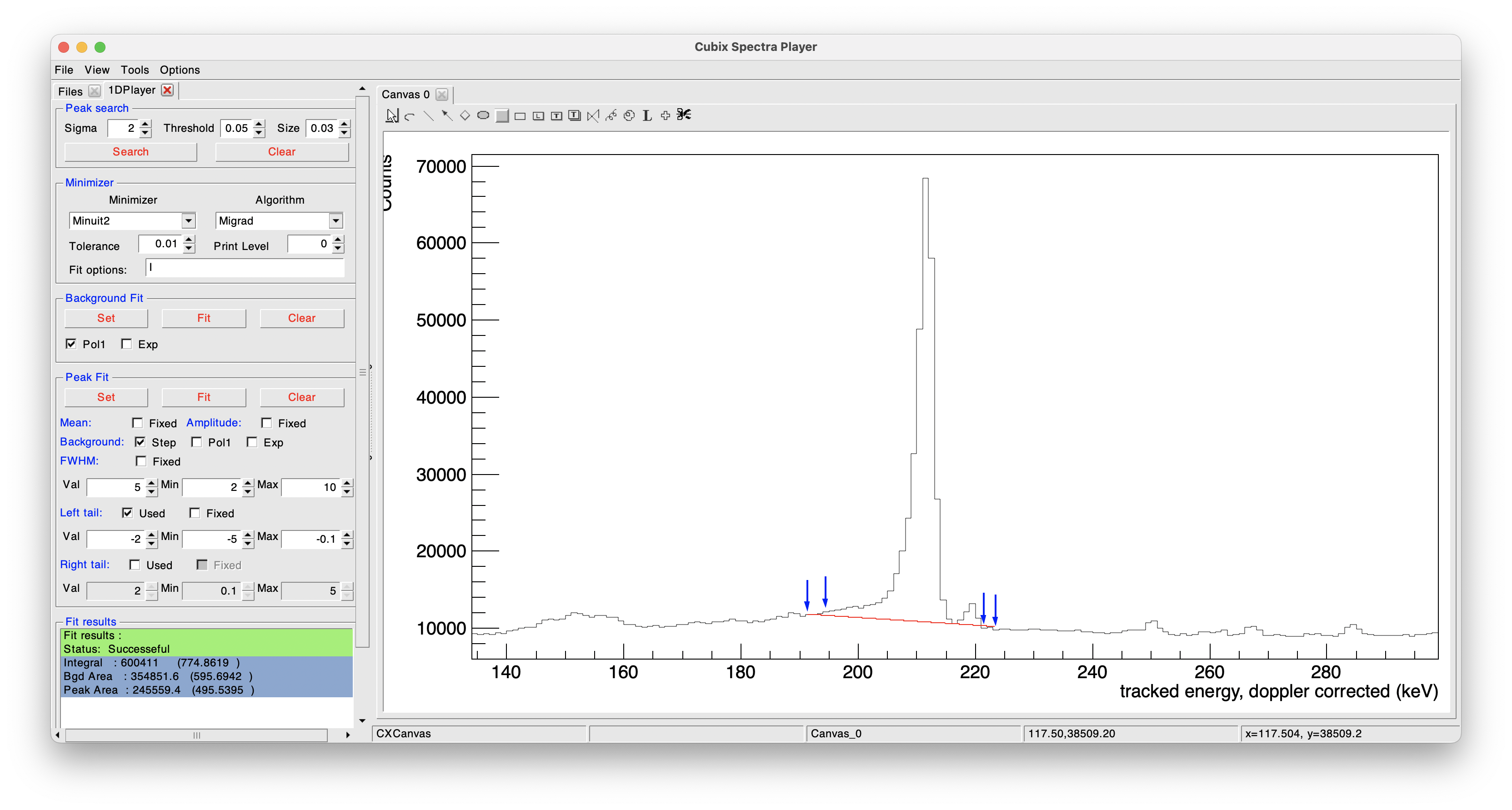
The obtained integral is printed in the terminal and in the cubix window.
- PeakFit:
The peak fit allows to fit a gaussian peak. As this software is dedicated to \(\gamma\)-ray spectroscopy, the default function suppose a gaussian peak, with a possible left and right tail (for taking into account possible neutron damage in the detectors or lifetime effects), and a step background to take into account the Compton part bellow the peak.
To define a peak (or multpiple peaks), you need to click on Set and then click on the positions of the background range (before and after the peak(s)). The order is not important, the lowest/highest values will be taken as background, and all the others arrows will be considered as peaks. Click then on Fit to perform the fit:
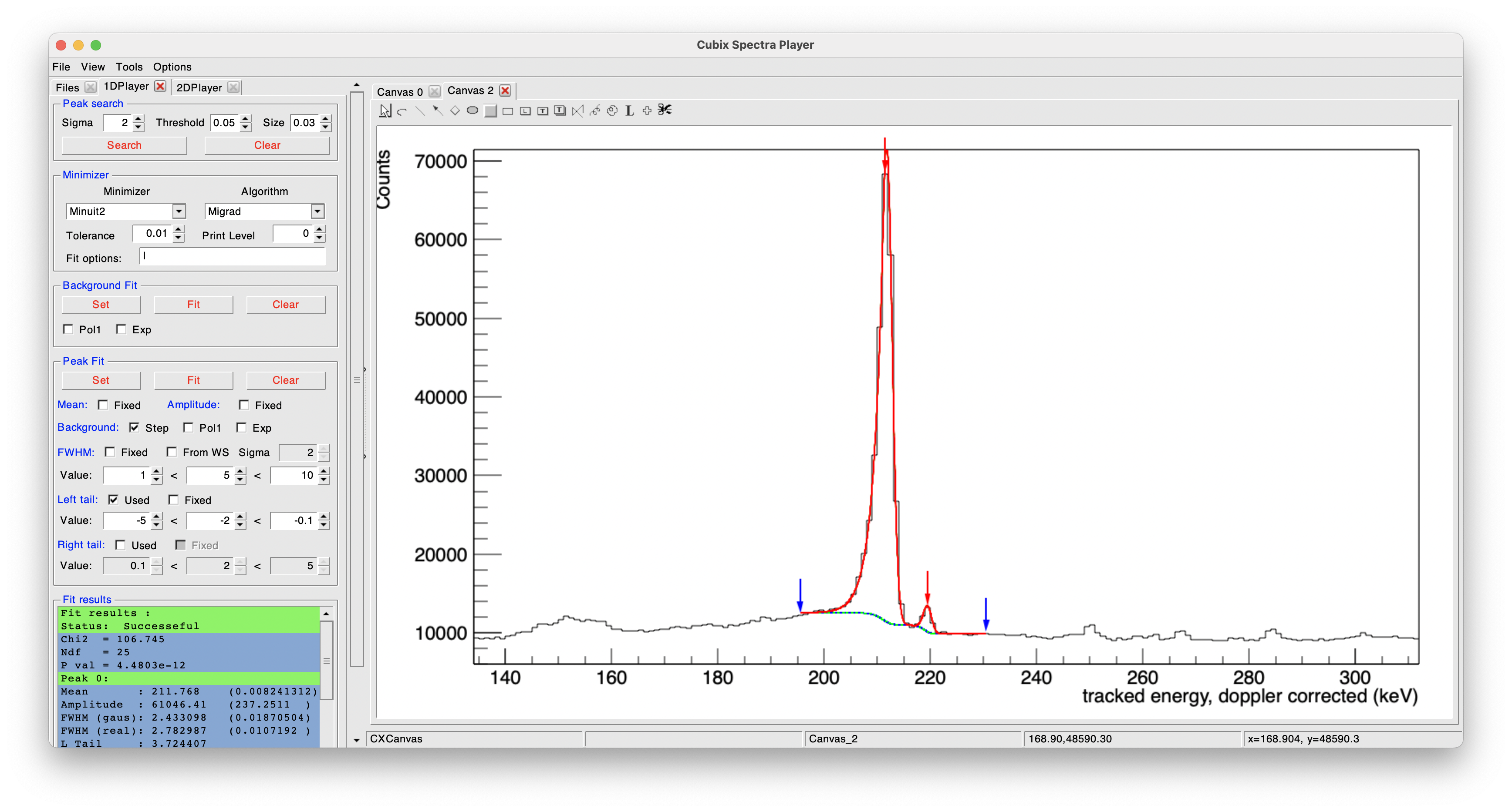
The following parameters can be defined:
- Mean: fix the peak centroid to the arrow value
- Amplitude: fix the maximal amplitude to one of the histogram at the arrow position
- Background: (multiple options possible)
- Step: stepped function bellow the peak (default)
- Pol1: polynomial function of order 1 (ax+b)
- Exp: exponential background
- FWHM:
- Fixed: Fix the FWHM at the defined value
- From WS: Use the FWHM function of the detector (if defined in the current Workspace)
- Sigma: If From workspace is activated, define the number of sigma to take as FWHM uncertainty
- Range: define the limits for the FWHM (if not using the workspace FWHM function)
- Left tail:
- Used: Fit with a left tail
- Fixed: Fix the left tail at the value defined bellow
- Range: define the limits for the left tail
- Right tail: (identical to left tail)
If the efficiency function is defined in the current workspace, the peak areas will be printed as real counts and corrected from efficiency in the terminal and in the cubix window.
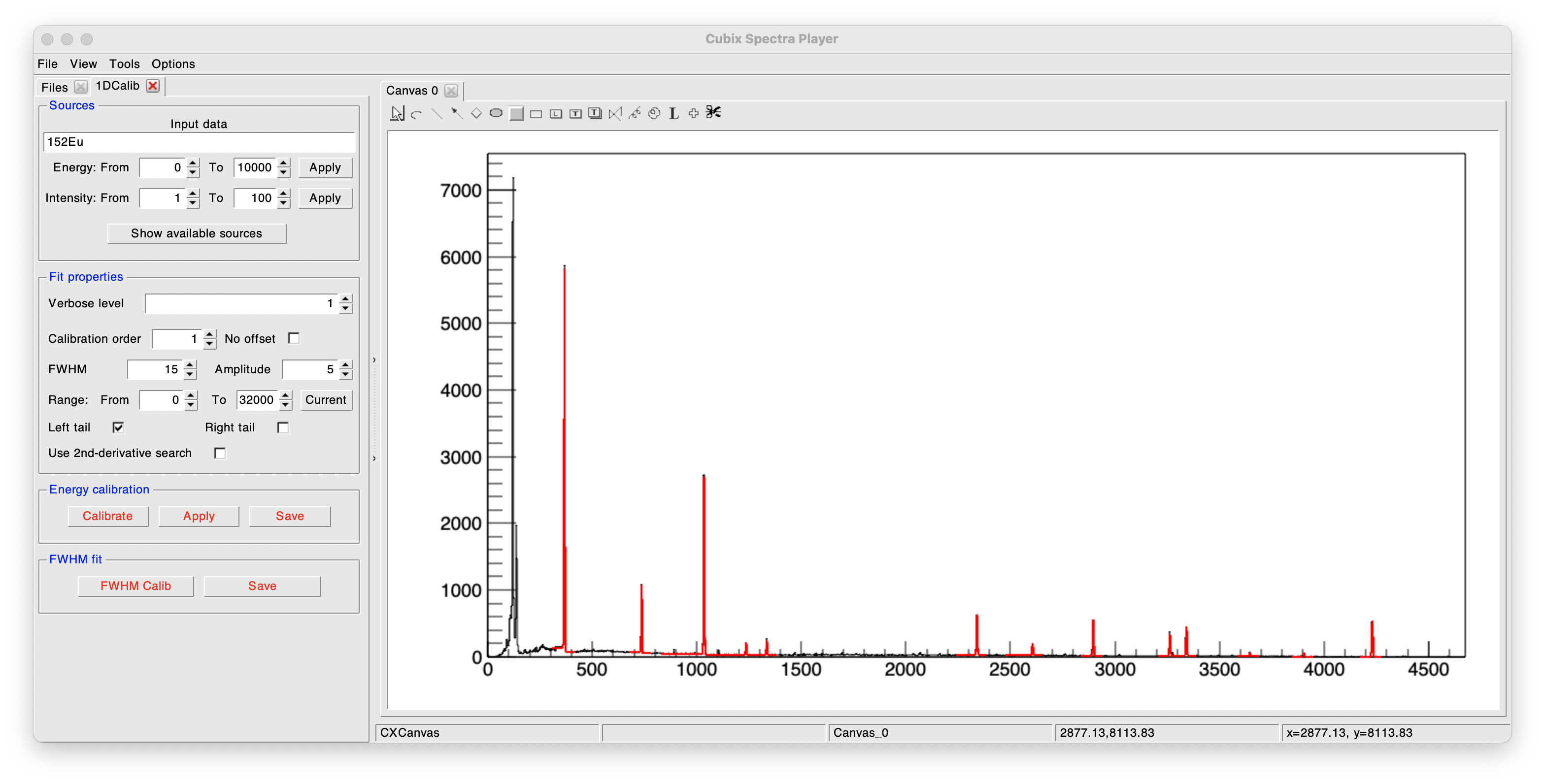
Energy calibration#
The energy calibration utility is used to determine the energy calibration parameters of a \(\gamma\)-ray spectrum. This is done using the original RecalEnergy program of the AGATA collaboration developped by Dino Bazzacco. It can also be used to extract and fit the resolution function that can then be used in the detector's Workspace.
source definition#
To show the availaible sources, click on Show available sources, this will print in the terminal such a message:
-- INFO    : Sources availbale (including intensities):
133Ba 134Cs 152Eu 22Na 241Am 56Co 57Co 60Co 88Y
-- INFO    : Calibration dataset availbale (only energies):
137Cs 208Pb 226Ra 28Al 40K
The sources that are including intensities can be used for efficiency fits (see Efficiency fits). For energy calibrations, all sources can be used.
The source files used are in $CUBIX_SYS/databases/Sources and can be adapted/modified/created. Here is an example of the 152Eu.sou source file:
#Generated from http://www.nndc.bnl.gov/nudat3/indx_dec.jsp with conditions:
#
#Nucleus             = 152Eu
#T1/2                > 1y && < 1e10y
#DecayMode           = Disabled
#Radiation Type      = Gamma
#Radiation energy    > 10keV && < 10000keV
#Radiation intensity > 0.1% && < 100%
#Ordering            = Z, A, T1/2, E
#Output              = Formated File
#Uncertainties       = Standard style
#
Dec Mode    Daughter    Rad Ene.    Unc         Rad Int.    Unc
EC          152SM       121.7817    3.0E-4      28.53       0.16
EC          152SM       244.6974    8.0E-4      7.55        0.04
EC          152SM       295.9387    0.0017      0.440       0.004
EC          152SM       329.41      0.05        0.1213      0.0024
B-          152GD       344.2785    0.0012      26.59       0.2
B-          152GD       367.7891    0.002       0.859       0.006
B-          152GD       411.1165    0.0012      2.237       0.013
EC          152SM       416.02      0.03        0.1088      0.0019
EC          152SM       443.9606    0.0016      2.827       0.014
EC          152SM       444.01      0.17        0.298       0.011
EC          152SM       488.6792    0.002       0.414       0.003
B-          152GD       503.467     0.009       0.1524      0.002
EC          152SM       563.986     0.005       0.494       0.005
EC          152SM       566.438     0.006       0.131       0.003
B-          152GD       586.2648    0.0026      0.455       0.004
EC          152SM       656.489     0.005       0.1441      0.0022
EC          152SM       674.64      0.14        0.169       0.003
B-          152GD       678.623     0.005       0.473       0.004
EC          152SM       688.670     0.005       0.856       0.006
EC          152SM       719.346     0.007       0.250       0.008
B-          152GD       764.88      0.04        0.189       0.004
B-          152GD       778.9045    0.0024      12.93       0.08
EC          152SM       810.451     0.005       0.317       0.003
EC          152SM       841.574     0.005       0.168       0.003
EC          152SM       867.380     0.003       4.23        0.03
EC          152SM       919.337     0.004       0.419       0.005
EC          152SM       926.31      0.05        0.272       0.003
EC          152SM       963.367     0.007       0.140       0.006
EC          152SM       964.057     0.005       14.51       0.07
EC          152SM       1005.27     0.05        0.659       0.011
EC          152SM       1085.837    0.01        10.11       0.05
B-          152GD       1089.737    0.005       1.734       0.011
B-          152GD       1109.18     0.05        0.189       0.006
EC          152SM       1112.076    0.003       13.67       0.08
EC          152SM       1212.948    0.011       1.415       0.008
EC          152SM       1249.94     0.05        0.187       0.003
EC          152SM       1292.78     0.05        0.101       0.003
B-          152GD       1299.142    0.008       1.633       0.011
EC          152SM       1408.013*   0.003       20.87       0.09
EC          152SM       1457.643    0.011       0.497       0.004
EC          152SM       1528.10     0.04        0.279       0.003
This ".sou" extension file is for sources with intensities (for efficiency fits, see Efficiency fits).
The ".cal" extensions are much more simpler, this is only a list of energies, as in the following example of \(^{28}\)Al source:
30.6382
104.62
212.017
271.175
314.733
831.45
846.764
983.02
1622.87
1778.969
1810.726
2282.773
2590.244
3033.89
3465.07
4133.408
4259.539
4733.847
6702.034
7213.034
7724.034
an energy can be commented using a "#". For printouts, a reference peak is used. By default this is the highest energy value. It can be changed adding a "*" after the energy of the desired \(\gamma\)-ray in the source file (see in the \(^{252}\)Eu exemple for 1408 keV transition).
Once one or more source has been defined in the Input Data text entry, it is possible to manually add energies by adding " -ener E" in the text entry. It is also possible to remove entries by adding " -remove E". The energy needs to be given with a precision of 1 keV to be removed.
Finally, it is possible to manually define the reference peak by adding " -ref E" in the text entry, here also with a precision of 1 keV.
fit options#
Some fit properties can then be defined:
- Verbose: define the verbosity of the fit process:
- 0: only print the calibration parameters
- 1: print the fit options summary and the results on the reference peak
- 2: print the results on all the peaks that have been found
- 3: print also the residues of each peaks
- Calibration order: define the calibration polynomial order to be applied. Select "No offset" to remove the order 0 offset (a0)
- FWHM: width used for the peak search
- Amplitude: given in %, minimal amplitude of a peak to be taken into account
- Range: range to be used for the peak search (click on "Current" to apply the current range)
- Tails: apply or not left/right tails in the peak fit
- 2nd derrivative search: Can be used in case of complicated peak search
calibration#
Clicking on the "Calibrate" button will print the fit results of each peaks:
It will also open a new canvas showing on the top the calibration function and bellow the residual plot:

Finally, the output, as a function of the verbosity selected, will be printed in the terminal:

Clicking on the Apply button will apply the current calibration.
Clicking on the Save button will save the current calibration function in the desired Workspace.
Resolution fit#
It is also possible to fit the detector's resolution by clicking on the FWHM Calib buton:

Clicking on the Save button will save the current FWHM function in the desired Workspace.
Efficiency fit#
The efficiency fit utility is used to determine the response function of the detector as a function of the energy. The function used is the one off the Radware program defined as:
\(Eff = Scale \times \exp{ [ (A+B*x+C*x^{2})^{-G} + (D+E*y+F*y^{2})^{-G} ]^{-1/G} }\), where \(x = log(E_{\gamma} / 100)\) and \(y = log(E_{\gamma} / 1000)\), with \(E_{\gamma}\) in keV
The \(Scale\) is a global scaling of the full function. \(A+B*x+C*x^{2}\) represents the low energy part (from 0 to the maximum of the curve). \(D+E*y+F*y^{2}\) represents the high energy part, and \(G\) corresponds to the curvature at the linking part between low and high energy parts.
source definition#
The source definition is the same than in the Energy calibration utility, with the limitation of only using ".sou" source files.
building efficiency curve#
If we want to fit the efficiency from a \(\gamma-ray\) spectrum, one first need to fit the peaks to build the efficiency curve. If we already have the efficiency curve and only need to fit it with the theoretical function, move to the section next section.
The peak search engine used behind is the same than for the Energy calibration utility.
The first step from a gamma source spectrum is to build the efficiency curve. This is done by clicking on Build eficiency curve. This will fit all the peaks of the selected source(s), determining its integral, and applying the source intensity of each transition to build the efficiency curve as:

A second window will be opened containing the efficiency curve:
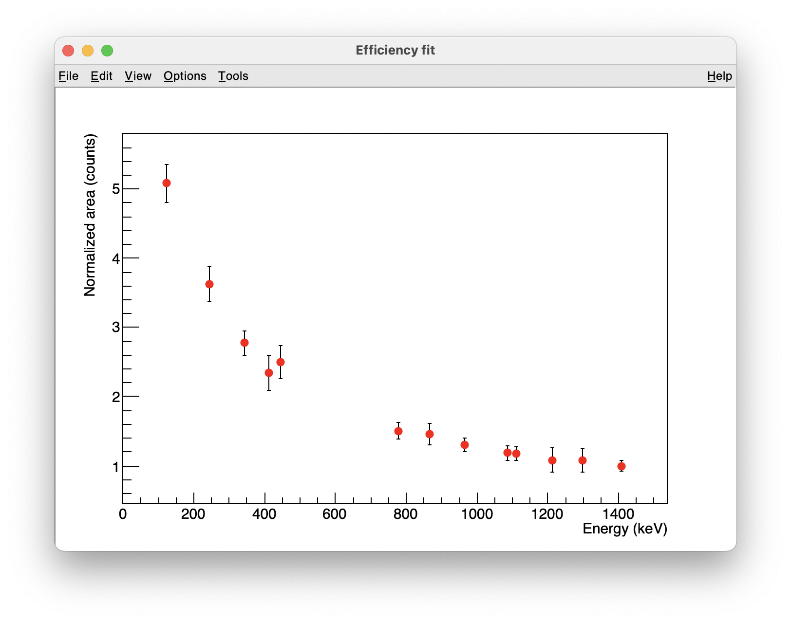
It has to be noted that this plot has been drawn with the option Normalize to ref enabled.
This means that the plot drawn is a relative efficiency plot, with a value set at 1 for the reference energy peak.
Fit efficiency curve#
Either the efficiency curve has been created as described above, either the curve has been already created outside cubix. In this latter case, one just need to open it with Cubix (TGraph format) and draw it in the current canvas.
To fit the efficiency curve, it is advised to use the Auto fit button that performs the minimisation in three steps: It first fits the low energy part, then the high energy part, and finally the curve linking both.
If the automatic process does not work as wanted, there is still the possibility to constrain manually the parameters and click on Fit for doing a single minimisation.
Once the fit is performed, the theoretical function and its error band is ploted. The following examples are showing the fit results obtained with and \(^{152}\)Eu (FIPPS array), and from a Geant4 calculation simulating a peak each 100 keV (AGATA array):
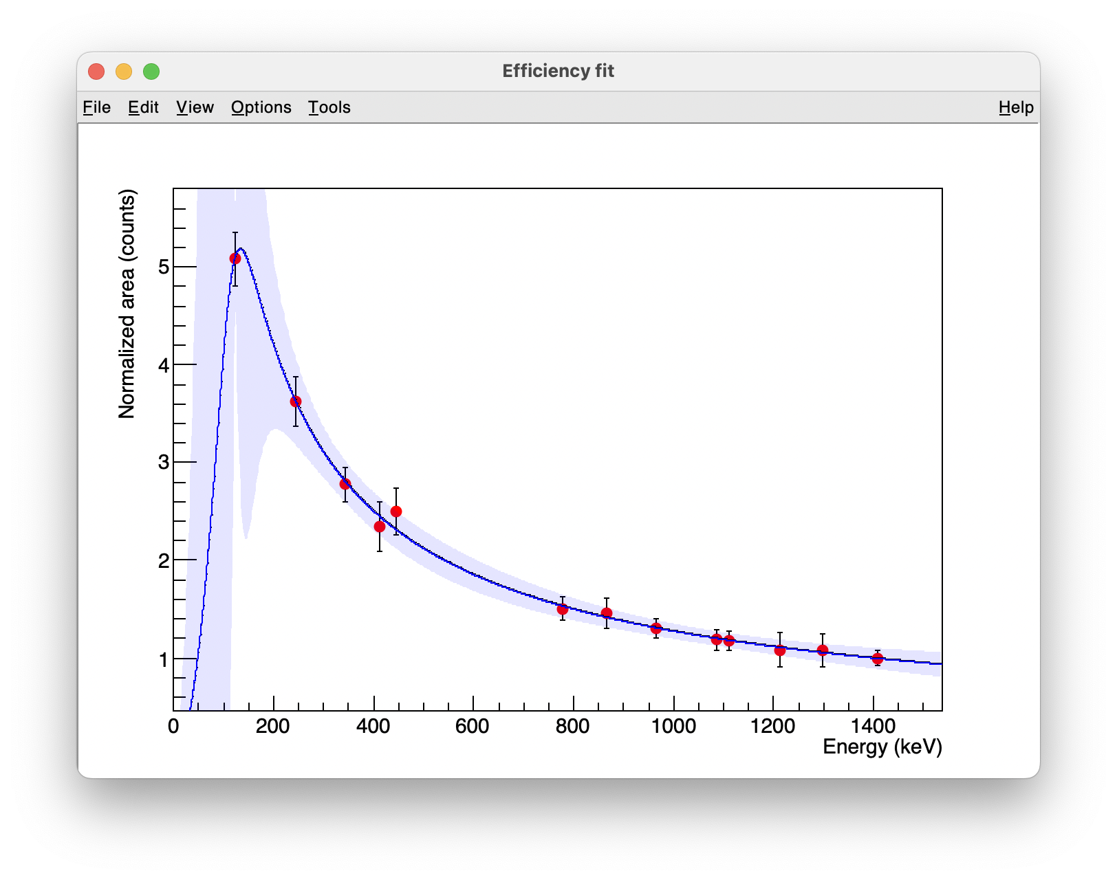
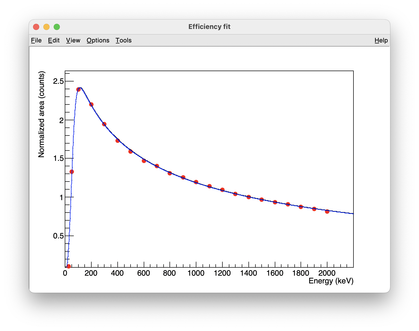
Once we are happy with the fit, it can be saved in a Workspace using the Save buton (see the workspace manager section for more details).
Background player#
The background spectra player allows for determining 1D and 2D backgrounds based on the ROOT TSpectrum classes.
- 1D background spectrum
When displaying a spectrum, click on "On" to show the standard background estimation. This can be adjusted by playing with the different parameters:
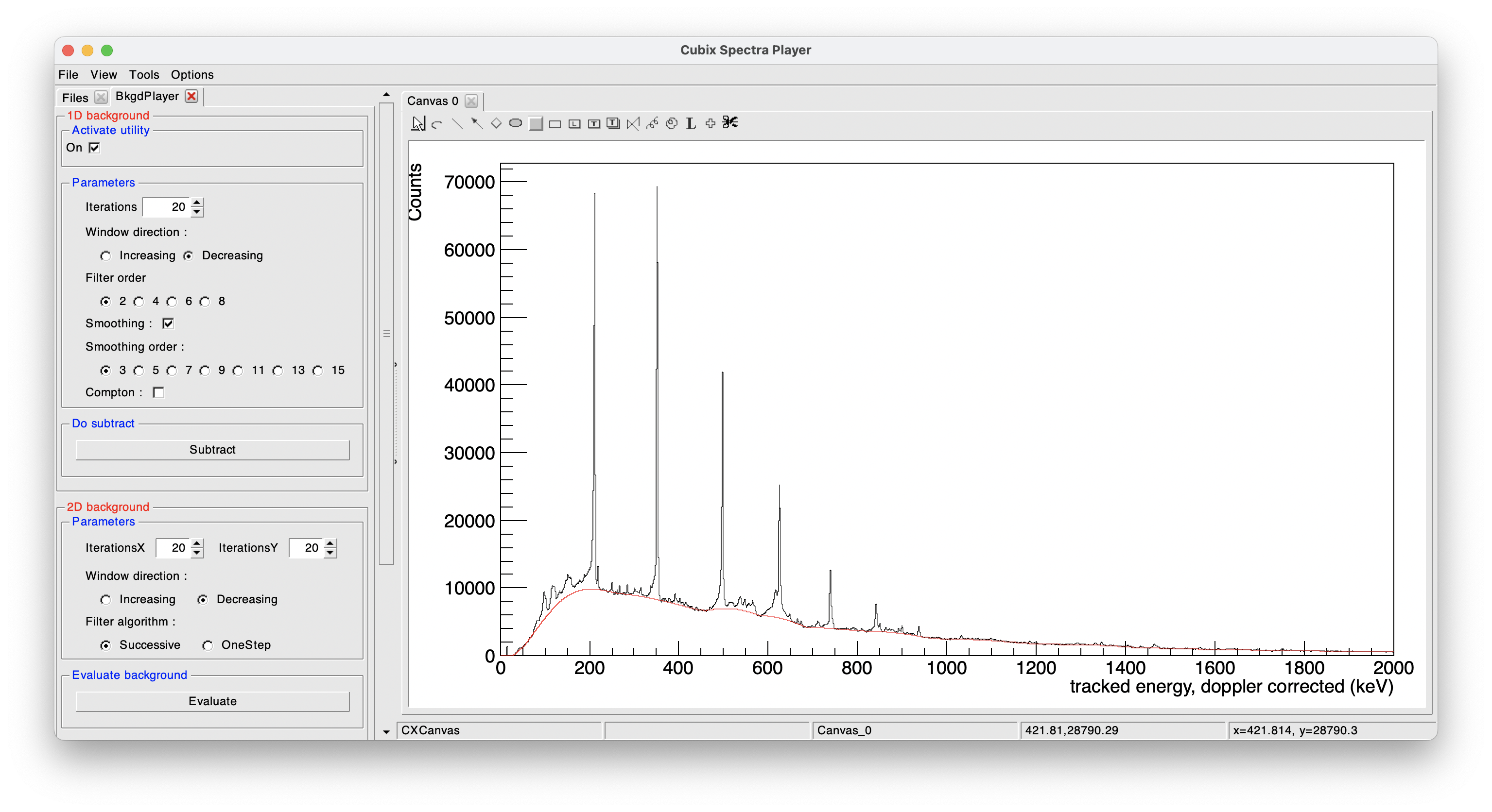
To subtract the background, click on "Subtract" and it will show the background subtracted spectrum:
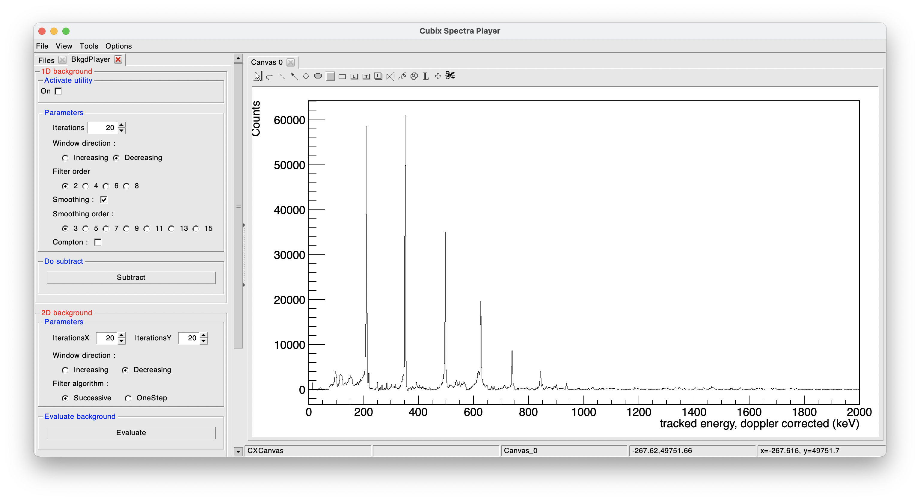
This tool need to be used carefully has this is a user-defined background. Peak area obtained on this kind of spectrum can differ to the one obtained on a fit performed on the original spectrum.
- 2D background spectrum
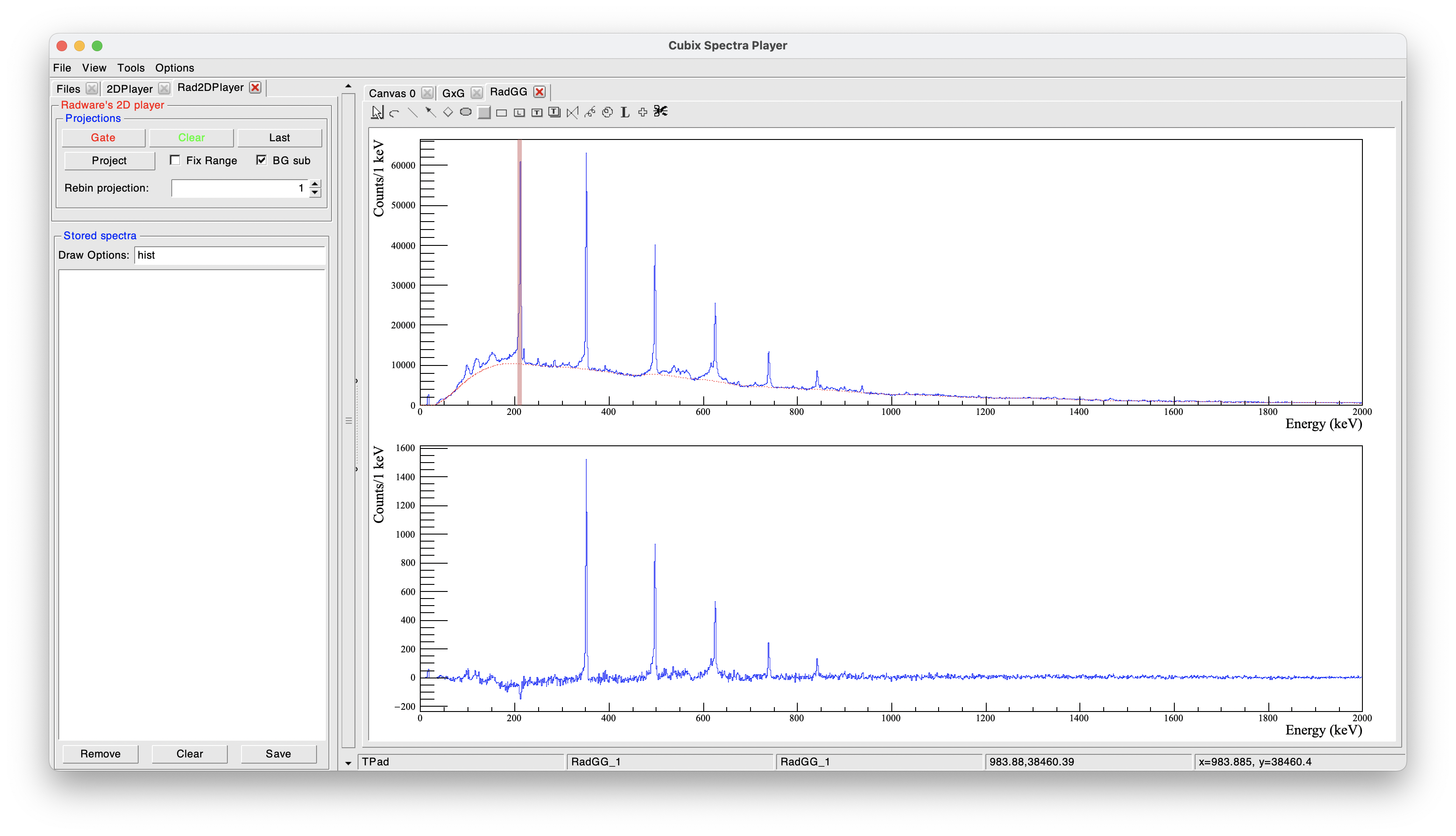
When displaying a 2D spectrum (namely a \(\gamma-\gamma\) matrix), click on "Evaluate" to start the 2D background evaluation. It will open a new canvas with on the top, the background subtracted 2D spectrum and bellow the remaining background:

The background subtracted 2D spectrum can then be used for a \(\gamma-\gamma\) analysis (see next section). Here again, be aware that the analysis quality can be affected by the way the background has been determined.
Angular correlation player#
The angular correlation player allows to plot the theoretical angular distribution between two correlated \(\gamma\)-rays, for given spins and mixing ratios.
It can also, for a given angular distribution that has been built from experimental data (in ROOT::TGraph format), fit the distribution to extract the experimental A2 and A4 parameters and perform the mixing analysis.
The player suppose a succession of two \(\gamma\)-rays, linking three levels of spins J1, J2 and J3 as in the following scheme:

The player looks like this:

The AngCorr tab is created after clicking on the New Instance button. It is composed of 4 sub canvases:
- top left: Theoretical distribution for the given spins and mixing value
- top right: 1D/2D mixing evaluation
- bottom left: display and fit of the experimental distribution
- bottom right: Chi2 minimisation of mixing values
When the AngCorr is open, double-clicking on a angular distribution in the TGraph format from the browser will directly plot this graph in the suited pad (botton left).
By default, we are assuming plots with an x axis in degrees.
If the experimental plot is in radians (range -1 ; 1 ), select the rad button before any fit of the distribution.
Correction factors setting/fitting#
Due to the finite size of the detectors, geometrical correction factors needs to be determine to be able to fit angular correlations with correct A2 and A4 values. If known, the correction factors can be defined in the left pannel. As these parameters are experiment dependant, it can be saved with the Save Qi button in a workspace for not having to set the values for each cubix use.
If these parameters are not known, this tool allows to fit them on already well known transitions.
It is advised to find a physics case for which the A2 parameter is strong, and another one where the A4 is strong (if you don't have one with strong A2 and A4 parameters).
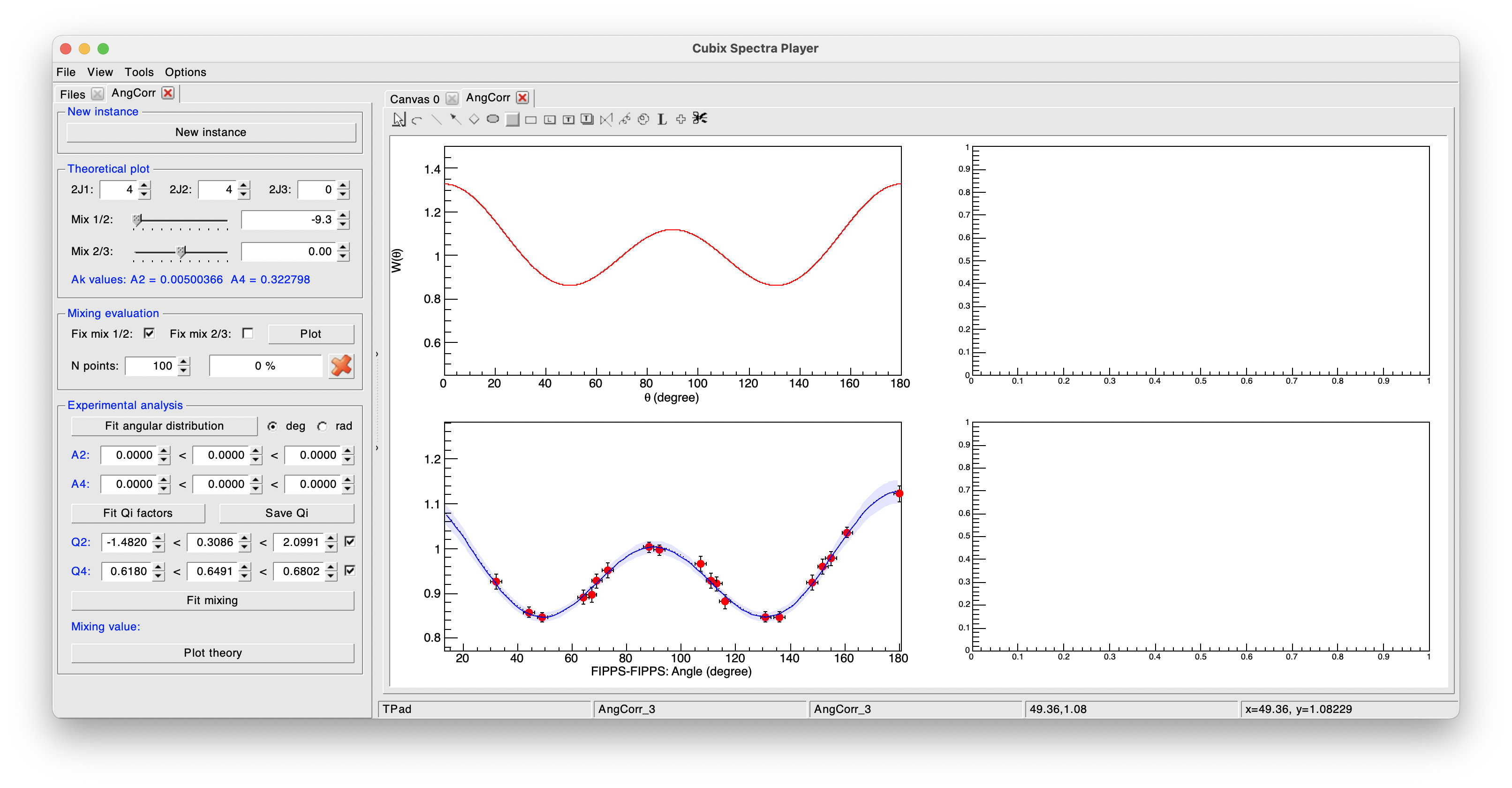
For example, here we will first fit the Q4 parameter on the transitions of 964 and 122 keV (\(2^{+}_{3} \rightarrow 2^{+}_{1} \rightarrow 0^{+}_{1}\)) of \(^{152}\)Sm measured from a \(^{152}\)Eu source.
The 964 keV transition has a known M1/E2 mixing of -9.3. We thus define in the player the spins and mixing value.
the spins needs to be defined as twice the spin (to have integer values for odd masses)
Once these values have been defined (see image bellow), the theoretical A2 and A4 values are shown in the left pannel. We can indeed see that for this kind of transition, the A2 value is almost 0. The Q4 fit is then done by clicking on the Fit Qi factors button:
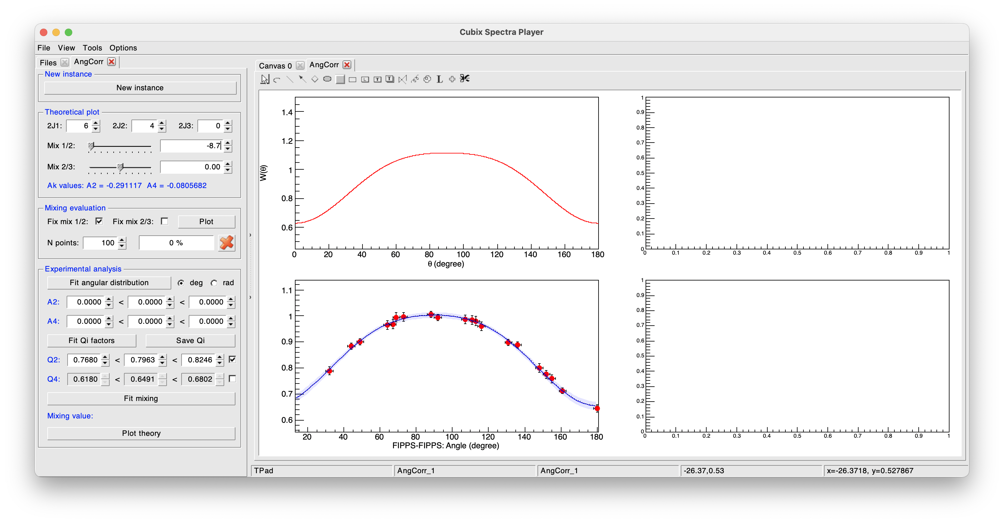
In a second step, we will fit the Q2 parameter on the transition of 1112 and 122 keV (\(3^{+}_{1} \rightarrow 2^{+}_{1} \rightarrow 0^{+}_{1}\)) of \(^{152}\)Sm measured from a \(^{152}\)Eu source. The 1112 keV transition has a known E2/M1 mixing of -8.7. We thus define in the player the spins and mixing value.
After setting these new values (see image bellow), we can see that here the theoretical A2 is much higher while A4 is almost 0. To keep the Q4 value of the previous fit, we unselect the Q4 line to fix its value in the fit process (see image bellow). The Q2 fit is then done by clicking on the Fit Qi factors button:
To check that the correction factors have been correctly defined, one can now fit the angular distribution by clicking on the Fit angular distribution button. This will update the experimental A2 and A4 values in the left pannel.
Once the correction factrors have been defined, it can be stored in a Workspace to be saved on disk and automatically load with cubix for other angular correlation anaylsis of the same experiment. This can be done using the Save Qi button.
To check the consistency of our results, we can perform a mixing analysis:
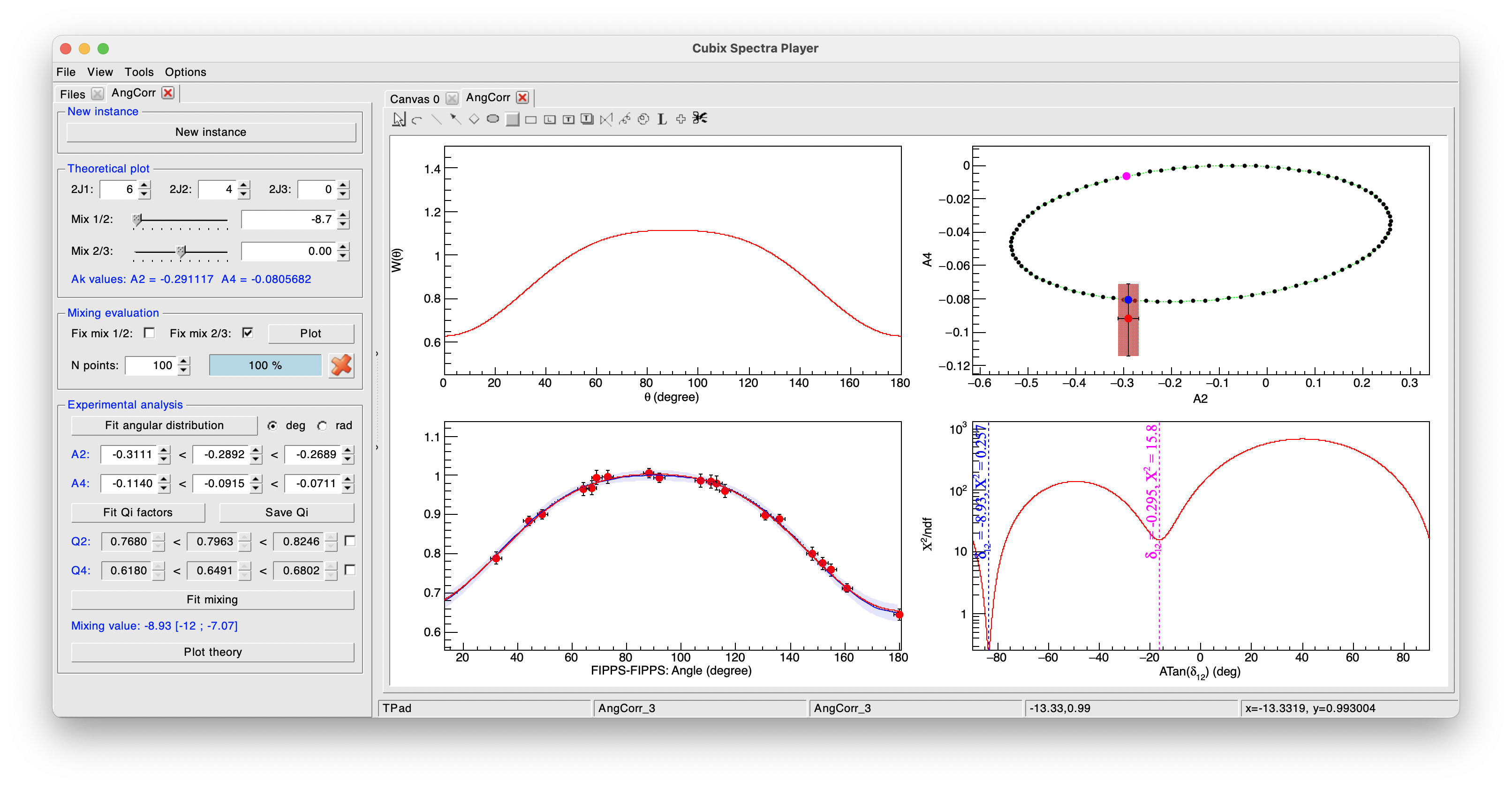
1D mixing#
If we already know the mixing value of a transition, we can fix it in the Mixing evalation part of the left pannel. Clicking on Plot will thus plot all the possible combinations of A2 and A4 for all the free mixing parameter in the top right pad. The experimental point will be overimposed and a green point is also drawn corresponding to the mixing value of the theoretical plot (it can be changed in real time).
It is then possible to perform a \(\chi^{2}\) minimization to calculate the optimal mixing value by clicking on the Fit mixing button. \(\chi^{2}\) plot will be drawn on the bottom right pad. The possible minimas will be shown with the corresponding mixing and \(\chi^{2}\) values. These minimas will also be reported on the top right pad to see what A2/A4 values it represents. The mixing value corresponding to the first minimum will be printed in the terminal and in the left pannel bellow the Fit mixing button. Its uncertainty can be calculated in two ways. If the theoretical values of A2/A4 values for this mixing value are within the experimental error bars, the mixing uncertainties are the limits of mixing values that allow to stay within the error bars. The other estimation is based on the \(\chi^{2}_{min}+1\) esimation. The mixing values, around the minimum, corresponding to a \(\chi^{2}\) of \(\chi^{2}_{min}+1\) are used as mixing uncertainty. These two uncertainties values are printed in the terminal.
Finally, it is possible to overlay on the experimental distribution the theoretical distribution corresponding to the current spins and mixing values by clicking on the Plot theory button. This will over impose the theoretical plot, renormalized to the A0 parameter of the experimental distribution and using the defined correction factors.
All these elements can be seen on the following figure:
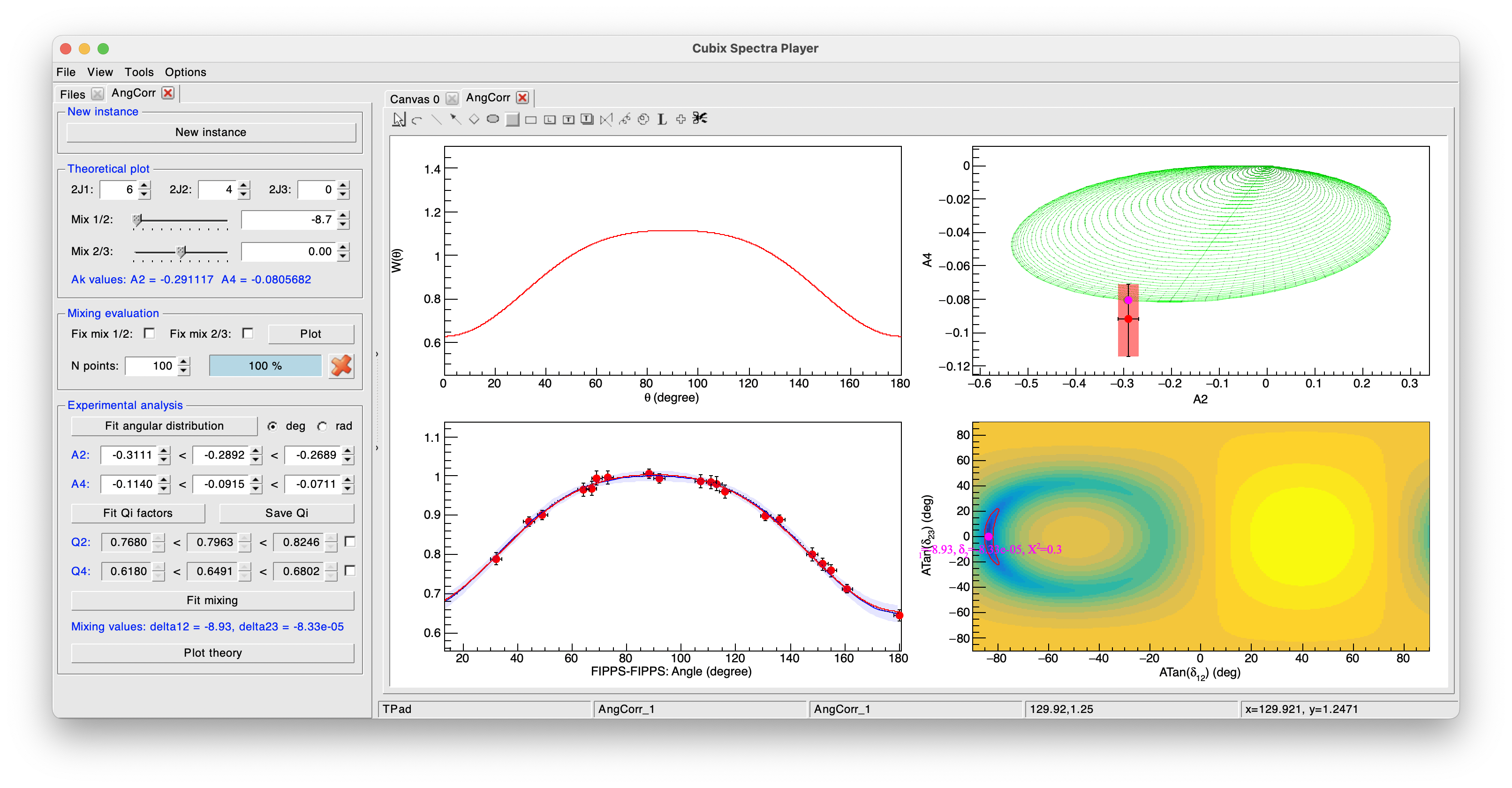
2D mixing#
If we don't know anything about the mixing value of both transitions, a 2D mixing can be done.
this kind of study will much likely give very large uncertainties because of the huge number of mixing combinations than can give the same A2/A4 values.
We need here to free both transition mixing in the Mixing evaluation part. Clicking on Plot will now represent a much more complicated graph of A2 and A4 combinations (see bellow).
Here again, we can then process the \(\chi^{2}\) 2D minimization to calculate the optimal mixing values by clicking on the Fit mixing button. The result will be a two dimensional function (one axis per transition mixing). The point corresponding to the lowest \(\chi^{2}\) is drawn with its corresponding mixing values. Here also, a \(\chi^{2}_{min}+1\) esimation is done. The contour corresponding to all values with a \(\chi^{2}\) of \(\chi^{2}_{min}+1\) is drawn in red. The mixing values corresponding to the lowest \(\chi^{2}\) are printed in the terminal and in the left pannel. No uncertainty is calculated at this level due to the complexity of its representation.
All these elements can be seen on the following figure:
examples#
Once the correction factors have been correctly defined, one can make the angular correlation study of other transitions. The following example is still from an \(^{152}Eu\) source: the transitions of 689 and 122 keV (\(2^{+}_{2} \rightarrow 2^{+}_{1} \rightarrow 0^{+}_{1}\)). The mixing of the 689 keV is known to be \(\delta(E2/M1) = +19 \pm 5\).
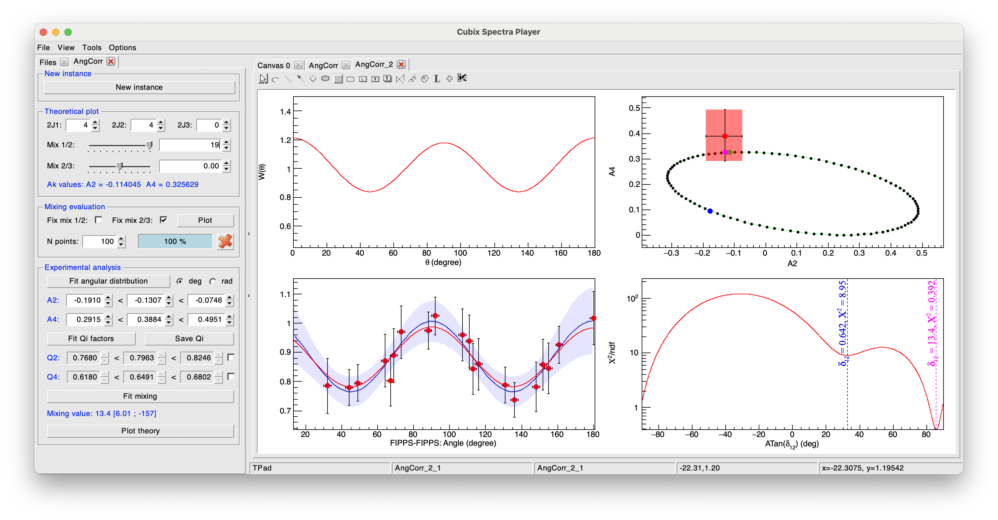
The results obtained is in good agreement with the literature with a mixing value determined as \(\delta(E2/M1) = +13.4 \pm 7.4\).
2D spectra utilities#
ɣ-ɣ player#
The \(\gamma-\gamma\) player is used based on a 2D histogram (\(\gamma-\gamma\) matrix) to make coincidence analysis. To start the player, either right click on an 2D histogram from the file browser and then select "Init GxG", or from a matrix already displayed in a canvas, right click on the matric and select "Init GxG". This will display the following view:
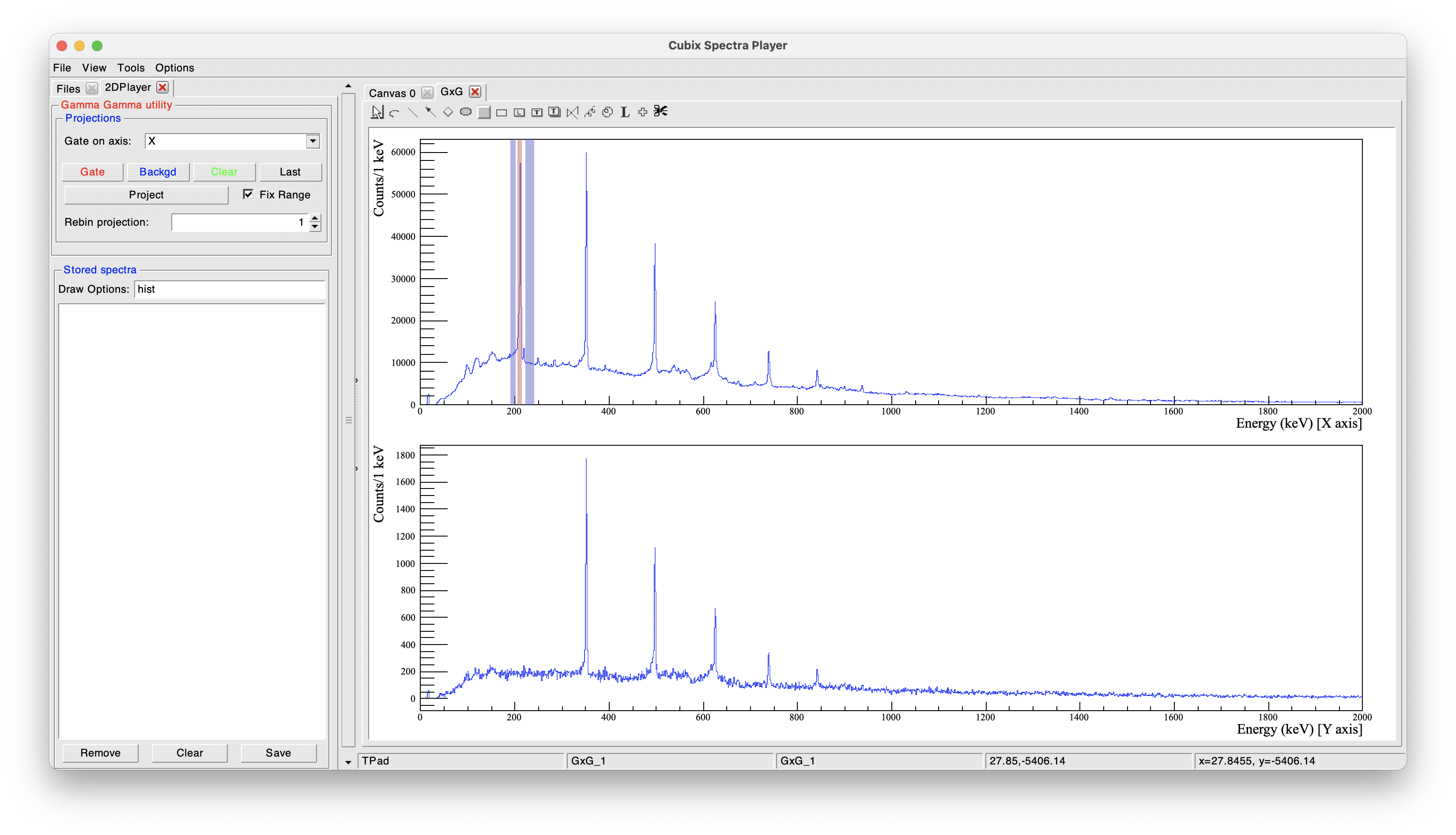
On the top right part, the total projection is shown (see bellow for the axis of the projection)
The bottom right part displays the projection according to the selected gates and background
On the top left part is located the pannel to define the gates:
- Gate on axis: to define (in the case of asymetric matrices), if the gates are done on X or Y axis (default gate on X, projection on Y)
- Gates buttons:
- Gate: Click on "Gate" to define a new gate. Once clicked, click, drag and drop on the total projection to create a red box.
- Background: Click on "Background" to define a new background. Once clicked, click, drag and drop on the total projection to create a blue box.
- Clear: Remove all the gates.
- Last: Apply the last gates configuration.
- Project: Calculate the projection according to the gates.
- Fix Range: If selected, the range of the projection will be kept as it is.
- Rebin projection: The projection will be drawn with a rebin of the histogram according to the selected value
On the bottom left part is shown the saved spectra utility (see Saved list utility). This can be here really usefull to store the projected spectra before doing a new gate.
As this is here not a 3D input, if more than one gate is applied, the result of the projection will be the sum of the gates (OR condition). More than one background can be defined for a single gate. It is advised to use one background before and one after the peak (as done in the example).
The background gates (blue) are not associated to a specific peak gate (red). The final projection is calculated as the sum of the individual gates minus the sum of the individual backgrounds, scales in a way that the total width of the backgrounds corresponds to the total width of the gates.
Options to define more precisely the gates:
- Once the gate is drawn, right click on it to define manually its centroid and width.
- Rather than using the buttons, right click on the total projection and select "Add Gate" or "Add Projection" and define the centroid and width
Keyboard shortcuts:
- Zoom utilities:
- Shift and drag and drop of the mouse to define the range
- CTRL + Shift and drag and drop of the mouse to define the range for the total projection and the gated spectrum at the same time
- Gates utilities:
- g to define a new gate from the graphical interface (as clicking on the "Gate" button)
- g + g to define a new gate by defining manually the centroid and width
- b to define a new background from the graphical interface (as clicking on the "Background" button)
- b + b to define a new background by defining manually the centroid and width
- d with the mouse on a gate to remove it
- p to project
ɣ-ɣ player (radware's style)#
The \(\gamma-\gamma\) player using the radware's style allows to do the same things than the standard \(\gamma-\gamma\) player but using the radware's way to make the background subtraction. When loading this utility (using "Init Radware GxG"), it will display the same kind of view than for the standard \(\gamma-\gamma\) utility:
As shown on this example, there is no more the possibility of adding background gates because the background is here automaticaly calculated. On the total projection, a background spectrum has been calculated (Radware's algorithm). It will be used to determine the background on the projected spectra. The background is first determine with the Radware's default parameters but can be adjusted by a right click on the total projection and selecting "SetBackground".
In this mode, the use of not symetrized matrices is not possible for the moment.
3D spectra utilities#
ɣ-ɣ-ɣ player (radware style)#
Cubix allows to create and read cubes using the Rarware's cube format.
Reading an already existing Radware's cube#
Let's suppose the cube main file is named "mycube.cub". Opening this file in cubix will try to load the following files:
- mycube.tab: file giving the binning definition (in Radware, a binning adapted to the detector resolution is ofter used). If no such file is found, a default one is taken.
- mycube.spe: total projection spectrum. If no such file, the total projection will be generated for the first read.
- mycube.2dp: 2D projection projection matrix. If no such file, it will be generated for the first read.
- mycube.bg.spe: background spectrum. If no such file, it will be automatically calculated.
- mycube.aca: energy calibration file. If no such file, cube will be supposed already calibrated
- mycube.aef: efficiency file. If no such file, efficiencies ignored (not used in the current version)
Another option is to define the file: "mycube.conf" containing all these links, as:
2DProj mycube.2dp
LUT mycube.tab
CalFile mycube.aca
TotalProj mycube.spe
EffFile mycube.eff
CompressFact 2
This second option allows to change more easilly the file names if needed, and allows to define the compression factor. This is to be used for binning of 0.5 keV/channel for example (Compression factor of 2)
To open a cube, double click on the file with the .cubextension. It will open the cube properties as follows:

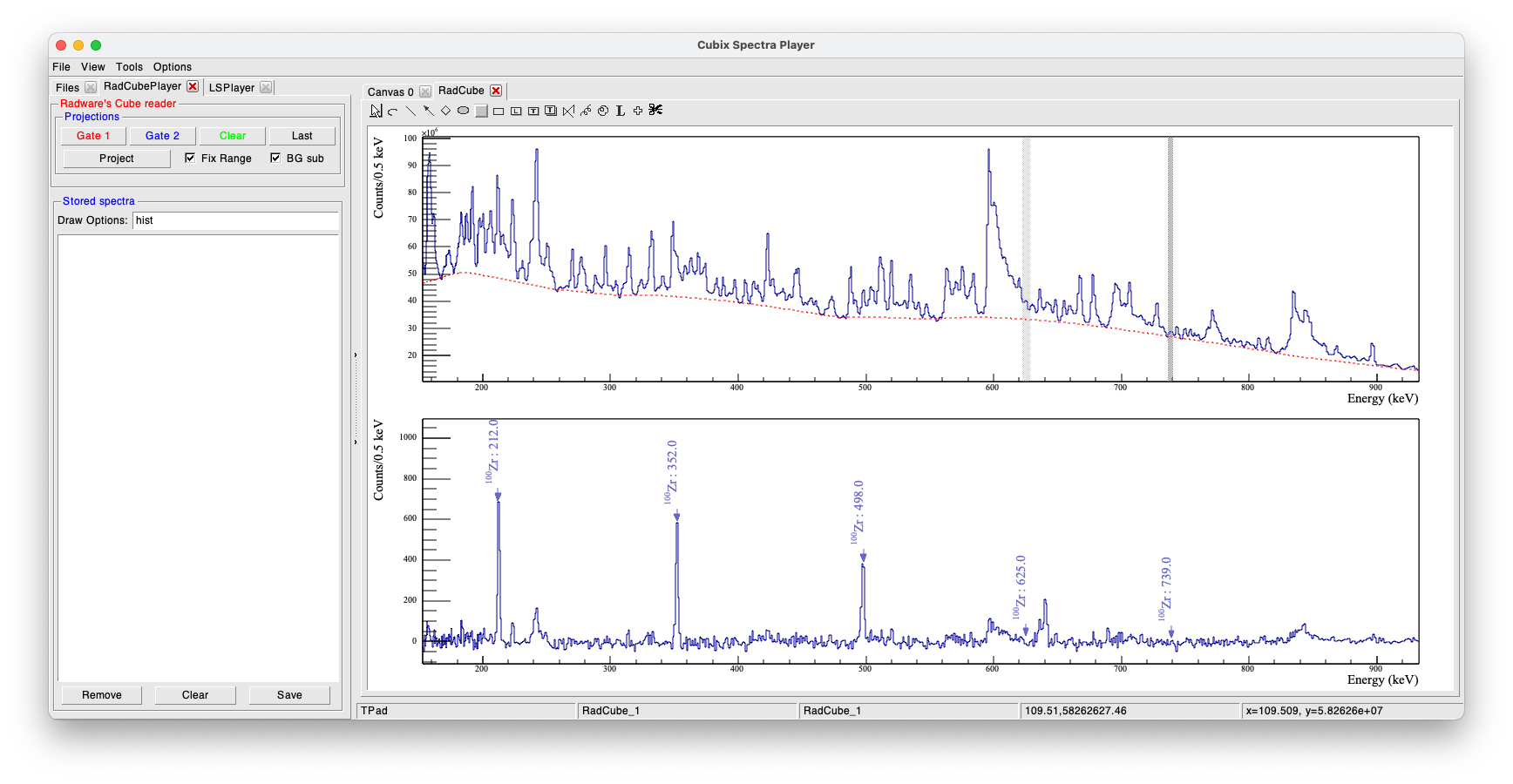
To load the cube player utility, double click on the Cube file (showed by the red arrow on the above picture)
As for the radware \(\gamma-\gamma\) player, we can put the gates by clicking on the buttons "Gate 1" and "Gate 2". The projection will make the gate(s) of Gate 1 AND Gate 2. In case of multiple gates, the combinations will be summed between "Gates 1" AND "Gates 2".
Keyboard shortcuts: * g + g to define a new "Gate 1" by defining manually the centroid and width * Shift + g + g to define a new "Gate 2" by defining manually the centroid and width
In the following example, we can see two gates set on \(10^{+} \rightarrow 8^{+}\) and \(8^{+} \rightarrow 6^{+}\) off \(^{100}\)Zr in a Radware's cube coming from fission data. We can clearly see in the projection the transitions in coincidence, namely the \(2^{+} \rightarrow 2^{+}\), \(4^{+} \rightarrow 2^{+}\) and \(6^{+} \rightarrow 4^{+}\).
Creating a cube from a TTree#
Cubix propose a program to build a cube in the Radware's format from a ROOT TTree. A cube configuration file needs to be defined as in the following example (an example of configuration file is located in $CUBIX_SYS/conf/CubeBuilder.conf:
#######################
### Cube Properties ###
#######################

# Name of the 3D cube file
CubeFileName MyCube
# Compression factor (to obtain binning <1 keV, one needs to scale the energy)
# For example, to obtain a minimal 0.5 KeV/Channel, we fill the Cube on 8k channel for 4keV range ==> Compression factor = 2
CompressionFactor 1

# Must be a power of 2. Max range of the cube
CubeSize 4096

# scratch file used as buffer in cube building in MB
ScratchSize 512

################################
## Input Root Tree Properties ##
################################

#Name of the input TTree (regular expressions can be used as for building TChain)
TreeFile E680_TTree_100Zr.root

#Name of the TTree
TreeName 100Zr_Z_40_A100

#Events to process (0 => All)
NEvents 0

#Name of the branch corresponding to the gamma-ray energy
EGamma EGammaDC

#Name of the branch corresponding to the gamma-ray muliplicity
GammaMult MGamma

#Cut to be apllied (see TTreeFormulaExpression)
Cut None
To create the cube, use the command:
CubeBuilder CubeBuilder.conf
This should produce an output like:
...
...Done creating new cube.
Axis length of 3d cube is 4096.
3d cube has 45001728 minicubes and 11009 records.
Making sure we have enough scratch space...
...Done.
Scan started:  Tue Nov  7 08:36:54 2023


-- INFO    : Input Tree reading to build the database...
Total 11405842 events |===================>| 99.72% [ 2.34e+06 evts/s, time left:   0h00min00s ]
-- INFO    : Building the cube...
...Updating cube from scratch file:  Tue Nov  7 08:37:02 2023

There are 5494 chunks to increment...
...
The process will end by creating the 1D and 2D projections of the cube. at the end you should have in your current folder the following files:
-rw-r--r--@ 1 dudouet  staff       1140  6 nov 11:32 CubeBuilder.conf   # configuration file for the CubeBuilder program
-rw-r--r--  1 dudouet  staff  536870912  7 nov 08:37 MyCube.scr     # temporary scratch file used to build the cube (size parametrized in CubeBuilder.conf)
-rw-r--r--  1 dudouet  staff        864  7 nov 08:37 MyCube.log     # log file of the cube building
-rw-r--r--  1 dudouet  staff   49090488  7 nov 08:37 MyCube.cub     # cube file to be open in cubix
-rw-r--r--  1 dudouet  staff   67108864  7 nov 08:37 MyCube.2dp     # 2D projection of the cube
-rw-r--r--  1 dudouet  staff      16424  7 nov 08:37 MyCube.spe     # 1D projection of the cube
-rw-r--r--  1 dudouet  staff         39  7 nov 08:37 MyCube.conf    # configuration file of the cube (to get the compression factor for example)
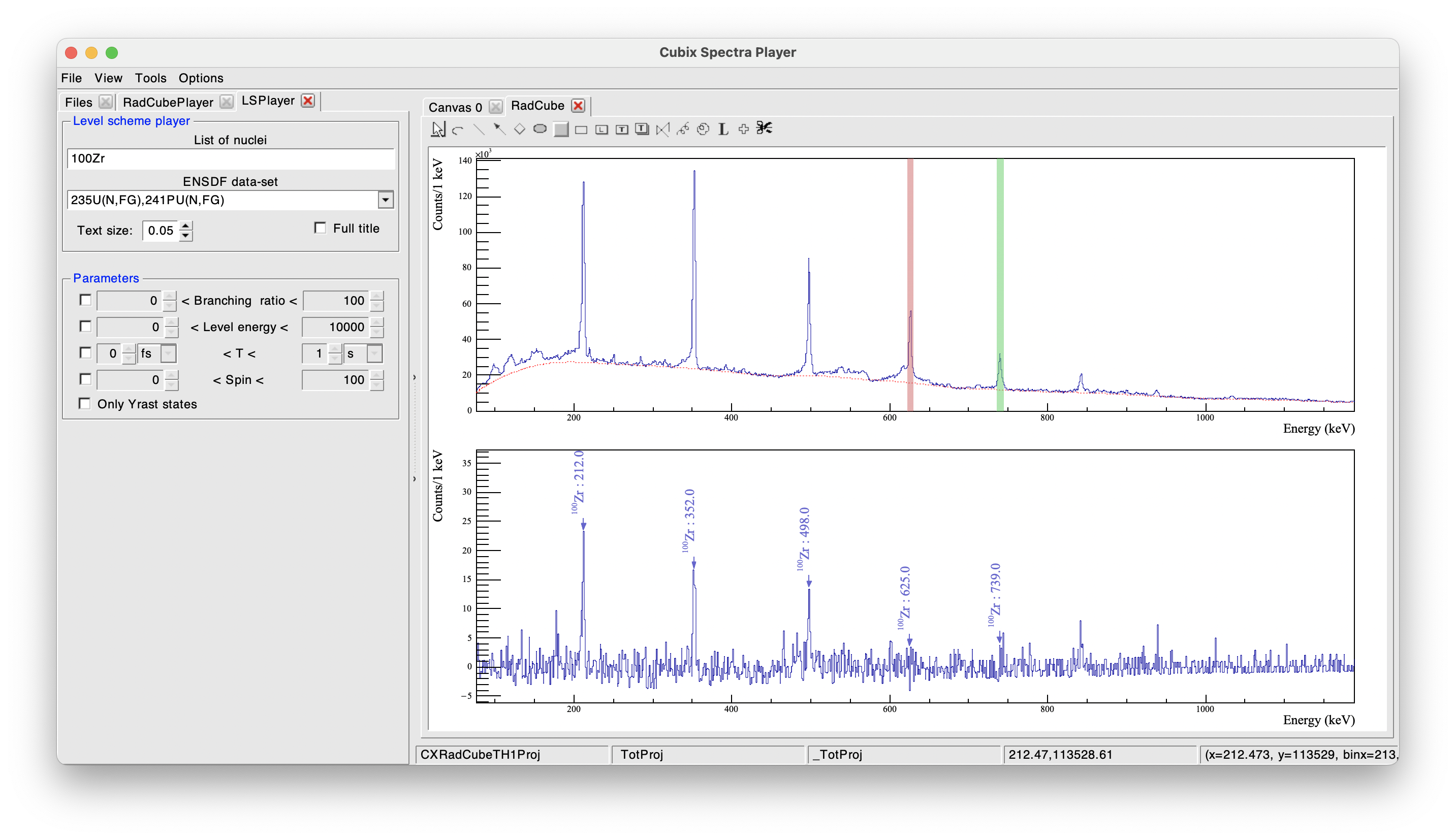
This new cube has been build from AGATA/VAMOS fission data filtered by VAMOS on 100Zr events. We can open it and apply the same gates than on the previous example:
Gamma search#
The gamma search utility allows to find in the database, to which nuclei can bellong the observed transitions. Up to three transition energies can be used and one can ask if these transitions need to be observed in coincidence or not.
In the following examples, we still use the 100Zr physics case. We can first ask which nuclei have in their level scheme transitions of 212(\(\pm\) 1) and 352(\(\pm\) 1) keV, in the given range of Z and N:
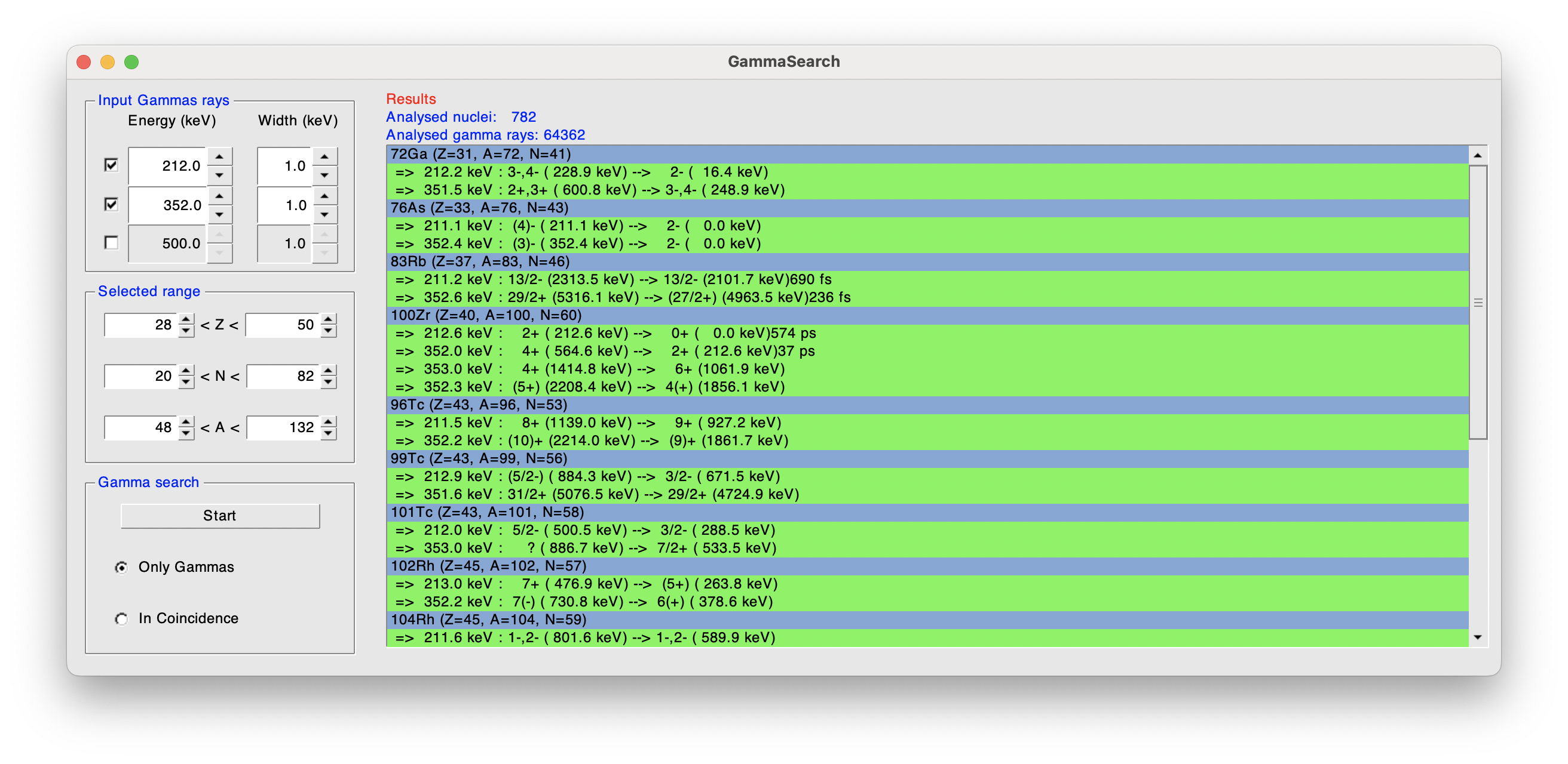
The full list is printed, giving for each nucleus, all the possible transitions corresponding to the request, sorted as a function of the parent level energy.
It is then possible to add the constraint that these transitions need to be in coincidence in the level scheme:
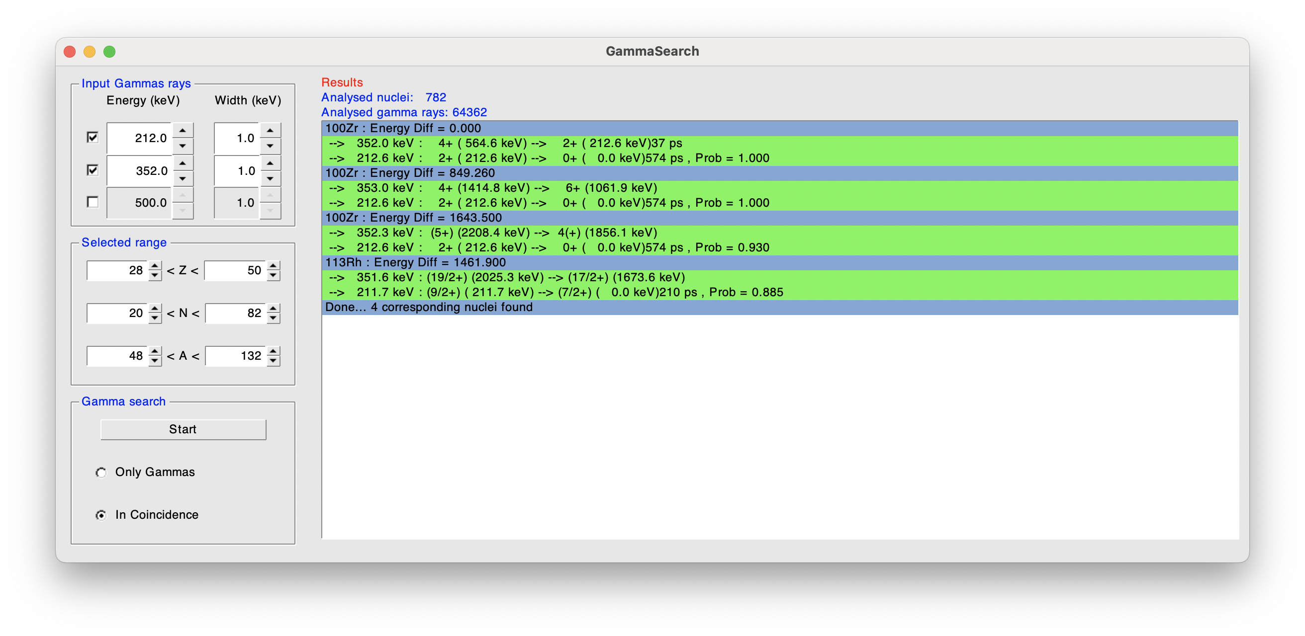
The list of possibilities is clearly shorter with this condition. An important point here is that for each given case, a probability factor is given. This probability factor is calculated as the successive branching ratio from the upper transition to the lower one. A probability of 1 means that, according to the database, all the decays corresponding the higher excitation energy will go the lower decay. The results are sorted, first by probability value, and then by the energy difference between the daughter level of the upper decay and the parent level of the lower decay. An energy difference of 0 means that the two decay are directly connected in the level scheme.
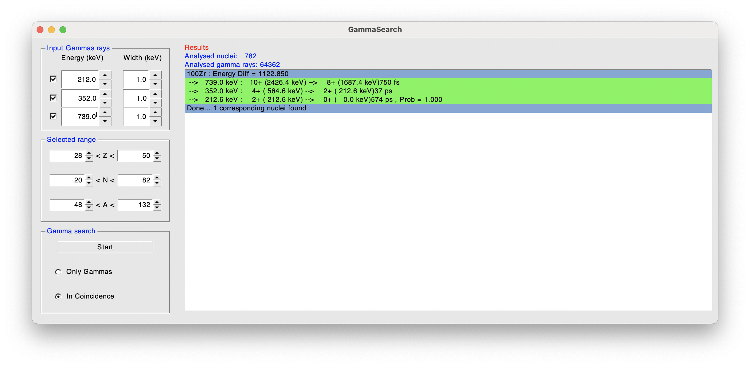
Finally, one can also ask for three decays in coincidence, adding in the following example the energy of the \(10^{+} \rightarrow 8^{+}\) transition in 100Zr:
Nuclear Chart Player#
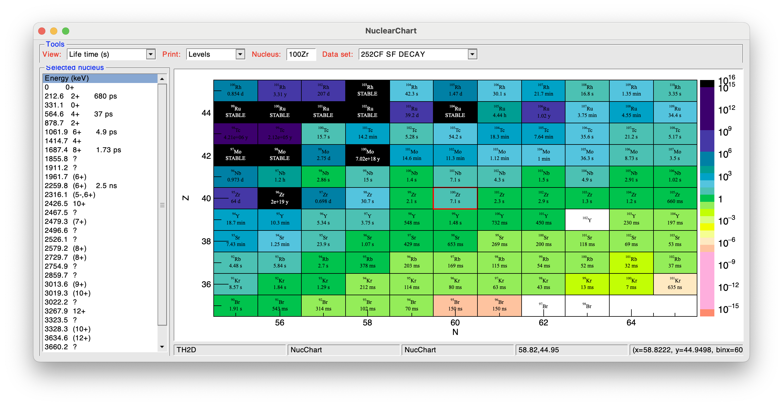
The nuclear chart player allows to plot some nuclear properties over the nuclear chart like:
- Ground state life time
- 1st and 2nd isomer life time
- 1st excited state energy
- Decay mode
- B(E2: \(2^{+}_{1} \rightarrow 0^{+}_{1}\)) in \(e^{2}b^{2}\) and Weisskopf unit
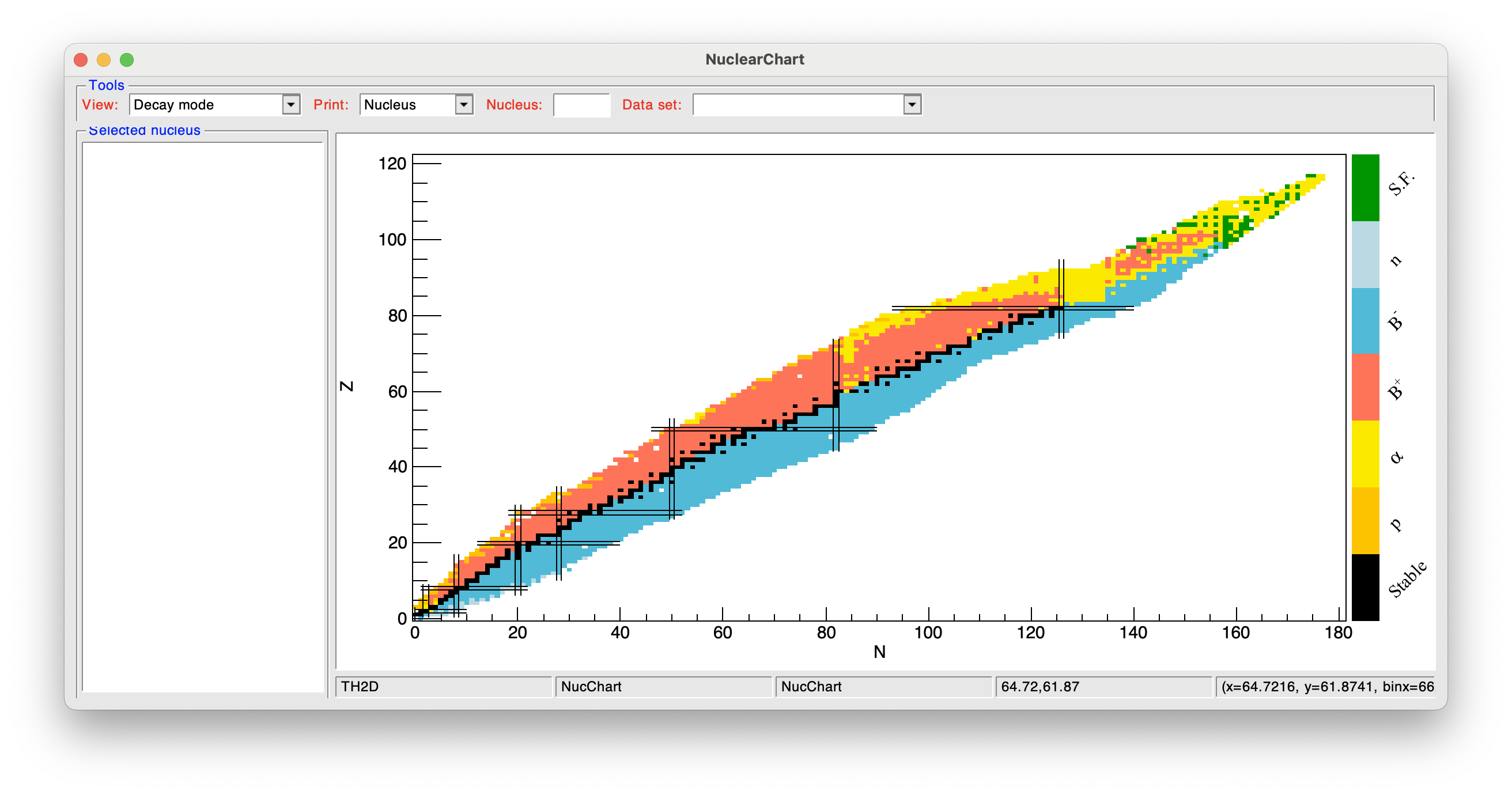
When selecting a nucleus (clicking on it, or writing its name in the Nucleus field will plot in the left pannel and in the terminal the selected information in:
- Nucleus ground state properties
- Nuclear level properties
- Nuclear \(\gamma\)-ray properties
The two last properties will be printed for the selected data-set: